The Maths of Fractal Landscapes and Procedural Landscape Generation
The purpose of this page is not so much to provide a mathematically complete and rigorous account of the techniques used for fractal landscape generation, but rather to provide an overview of these techniques and their application that is accessible to someone with high-school level maths. Those who have a more complete understanding of this field will notice that there are some complexities that are glossed over.
The Fractal Geometry of Nature
In conventional geometry, shapes are defined by simple formulae. Thus, an ellipse might be expressed as a function of radius and angle in polar coordinates. Such formulae are simple mappings - we put in a value of the angle in, we get a value of the radius out. We put a value for the radius in, we get 4 angles out in the range 0 -> 2p.
For a fractal object, this ceases to be the case. The key to fractals is that they have recursive definitions. In other words this means that, for example, the position of a each point on a fractal path is given by the sum of an infinite series. In most cases, this series has no analytic solution, so all we can hope to do is to converge on the correct solution by calculating successive terms in the series. An example of such a series is that which describes the Mandelbrot Set:
Zn+1 = Zn + C
Z and C are complex numbers. If we begin with Z0 = 0 + 0i and C = x + y i, and we calculate successive terms, |Z| (the size of Z) either becomes larger and rushes towards infinity, or it stays close to zero, trapped in a so-called basin of attraction. If it were possible to continue to n = INF, we would either find |ZINF| to be infinite, in which case the initial point, C, lies outside the set, or to be finite, in which case C lies inside the set.
Another sort of fractal is best described in geometric terms, using a rule of replacement. Such an example is the Koch Snowflake. It is described by a procedure:
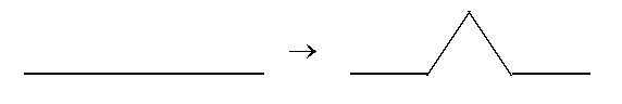
If we continue this for about 5 iterations, we get the following shape:
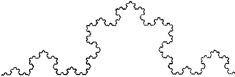
In the case of the Koch Snowflake (the above shows just the top - the full figure does resemble a snowflake) we have a recursive geometric description of the set, with each new approximation to the fractal a little closer to the final, infinitely complex shape.
To help us describe fractals, we use a measure called 'fractal dimension'. This is a measure of the increase in complexity at each iteration. In the case of a one-dimensional example such as the Koch Snowflake (where the fractal object is a perimeter rather than a surface), the fractal dimension is between 1.0 and 2.0. It is, if you like, a measure of roughness of the surface. We calculate it using the following formula:
Fractal Dimension = log(Length iteration n+1) / Log(Length iteration n)
The above replacement rule replaces a section of perimeter with a section 4/3 times the length. This gives us log 4 / log 3 = 1.26 as the fractal dimension of the curve.
If the fractal object is a surface, and it is displaced in a third dimension (i.e.: like a fractal landscape), then the fractal dimension is between 2.0 and 3.0.
Now we have the basic terms with which to describe fractals, we can examine some natural processes. Benoit Mandelbrot, beginning in the 1960s, observed and recorded the properties of many natural phenomena, from turbulence in fluids to the stock market. After twenty years of conducting investigations into the mathematics governing these traditionally intractable problems, he published a book called The Fractal Geometry of Nature, which describes how many natural phenomena follow the same sort of pattern as that observed in fractal functions.
Nature is not, however, fractal in the strict mathematical sense. No two trees are alike, and nor are any two mountains, but there is only one Koch Snowflake, one Mandelbrot set and so on. The best we can do is to say that natural processes have some characteristics which are similar to those of fractals. Once we have made such a connection, we can then use our measure of fractal dimension to describe the 'approximate fractal dimension' of a natural object.
Simulating Natural Objects
If we know that a particular type of object is approximately fractal in nature, and we wish to model it, we need to generate some parameterised model, incorporating features present in the real object (in particular, some sort of controlled randomness), without losing the controllability of the fractal model. The way we do this is using a 'random fractal' process. Instead of using a set geometric rule of replacement as we did with the Koch Snowflake, we generate different rules of replacement based on the values of the model's parameters, each of which differs from the others in some controlled random way.
This is exactly the process that we use to generate fractal landscapes. As soon as we introduce randomness into the equation, we can no longer talk about fractal dimension as an analytical property of the system. Instead, it becomes a statistical property, with a mean and a variance. However, we usually save ourselves the trouble, and quote mean fractal dimension.
Displacement Noise
There are two main ways to generate fractal surfaces that are widely used: displacement noise (described here) and gradient noise (the best-known examples of which are classic Perlin noise, and the more recent and better Simplex Noise). Here I will mainly examine displacement noise, with a view to removing the common issues that might arise from using it.
Subdivision and Displacement
There are several schemes which can be used to inject randomness into a fractal process, but fractal behaviour is not the only requirement for a believable landscape. Indeed, there is rather poor correlation between pure fractal processes and real landscapes. This means that it is necessary to post-process and possibly combine different fractals to achieve the desired result. Anyone who has ever used a photo-editing program will know that the higher the quality of the source, the greater the range of effects that can be achieved, and the same is true of fractals.
A 'high-quality' source fractal process is one which is stationary (all locations have the same statistical properties) and isometric (has the same properties in all directions). We could achieve both of these using a technique called Fourier synthesis, but this is extremely slow compared to other methods of generation. The reason why Fourier synthesis has such ideal properties is that the frequency spectrum of a landscape generated using this method is continuously variable - which is certainly true of natural ones as well. There is, however, almost no difference between a landscape generated this way, and one generated using a technique called recursive subdivision and displacement with cubic interpolation. The largest difference is a discrepancy in generation time of 20 times or more. With this in mind, I will not examine Fourier synthesis here.
The process of recursive subdivision and displacement is as follows:
We express the landscape as a grid of heights. For each 4 grid points, we work out the height of the points between them (interpolation), and then we add random values to all of them. One stage of this is shown below.
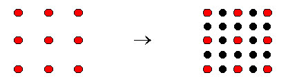
The red points represent the initial grid, and the black points represent the new points, whose heights are calculated by interpolation. All of these points then have random values added to them.
There exist a few different ways of calculating the heights of the new points. We can either just average the heights of the old points around them (linear interpolation) or we can try and follow the curve of the landscape a little more closely, using cubic interpolation. Typically, for cubic interpolation, you would use bicubic Catmull-Rom interpolation: but because the coordinates of the interpolated points are fixed, the necessary weights can be pre-calculated. Cubic interpolation has the advantage of continuity of gradient at the edges of the surface, meaning that there are no ugly horizontal and vertical ridges.
Controlling Fractal Dimension of the New Surface
As was mentioned previously, it is necessary to be able to control the fractal parameters of the surface. The most important of these is fractal dimension, which is a measure of how rough the landscape is. The fractal dimension of a fractal landscape must lie between 2.0 and 3.0. Outside these ranges, we cease to have fractal behaviour. For no reason other than simplicity, it is also decided that the mean fractal dimension of the landscapes we generate should be constant. It can be shown that a necessary and sufficient condition for constant mean fractal dimension is a frequency profile of:
Amplitude = 1 / frequencyb
Where beta is a constant for any given landscape. We can approximate this frequency profile by assuming that the frequency at any iteration of our subdivision scheme is given by the reciprocal of the smallest square size at that point in time.
There remains one thing to be done: we need to work out what range of values for beta will give rise to fractal dimensions between 2.0 and 3.0. As it turns out, they are related by the following formula:
Fractal Dimension = (7 - b)/2
This means that beta must be between 1.0 and 3.0. At b = 1.0, the system will only just converge (fractal dimension = 3.0), while at b = 3.0, the landscape would be very smooth indeed (fractal dimension = 2.0).
Non-Isotropic Behaviour and some Solutions
The simple subdivision algorithm already described, while quite powerful in some circumstances, does not behave quite ideally. The most noticeable artefact is that landscape features can appear somewhat square. This arises because the algorithm operates on a square grid, and the interpolation is not sufficient to remove all directional dependence. In other words, the landscape is not isotropic.
The Diamond-square algorithm is one frequently used solution to this problem. This works by subdividing the square grid into diamond-shaped sections, and the subdividing these into square-shaped sections again.
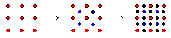
Thus, at each step, the interpolated position of one of the new points depends on exactly four other points.
Unfortunately, while it seems like a good idea on paper, this is largely unnecessary with proper interpolation on a regular grid.
Deviations from Natural Landscapes
Assuming we make a surface using vertical displacement on a square grid as described here, with cubic interpolation, there are some key ways in which the resulting surface will deviate from a real landscape.
Gradient Limitation
For a given set of parameters, there is a maximum gradient of the resulting surface. Real landscapes, however, have places where the gradient is infinite (cliffs).
Anisotropy
It can easily be seen from the geometry of a regular grid that the direction of maximum gradient will always be aligned to the lines of the grid used to generate the landscape, regardless of the type of interpolation used. This is a noticeable and physically unrealistic situation, which will tend to make valleys and mountains run north-south or east-west, whereas their directions should be random overall.
Local Minima
Given enough time for erosive processes to act on a real landscape, local minima are extremely rare. This is for two reasons. One is that the erosive processes that shape a real landscape are almost always more significant on steeper terrain. This means that, with few exceptions, flat terrain will not be vertically eroded, and therefore minima will not generally develop. The one exception is that glaciers can vertically erode their bases, creating lakes. The other reason is that, in the absence of active geology, these natural lakes are both rare and transitory: in a reasonably short geological timeframe, most lakes will be filled in by sediment.
The displacement noise method of creating a landscape will lead to approximately equal numbers of maximum (mountains) and minima (lakes or isolated hollows) which is very far from being physically realistic.
Stationarity
One of the key ways a fractal landscape differs from a real landscape is that real landscapes have different statistical properties at different locations. The great plains of the US look very different to the Rocky Mountains, for instance. The process above will generate a terrain with a single set of statistical properties: meaning that you either have mountains or you don't. This property is called stationarity.
A Method for Fixing Anisotropy and Gradient Limitations
The first two of these issues are very straightforwardly fixed by allowing horizontal displacement in the interpolation step. Suppose, instead of simply displacing each vertex vertically, we also displace it horizontally. This would then tend to create both a random direction of maximum gradient and remove the gradient limitation of the resulting surface.
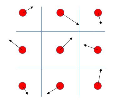
The issue with this solution is that, for the purposes of simplicity, we really, really want the output of the process to be a regular grid. We can, however, invert the problem. Rather than displacing the grid points, we can leave them fixed, but take their heights from a different location on the generated bicubic surface. This is equivalent to allowing the grid points to move, but then re-sampling back to a regular grid afterwards. An illustration of this is shown below.
The full process then becomes:
- Displace the grid points.
- Randomly choose a location on the resulting bicubic surface within the part of the grid nearest to each point, and make a new surface from these heights.
- Subdivide the new surface using bicubic interpolation as before.
This obviously doesn't have quite as strong an effect as moving the grid points themselves, but goes a long way towards correcting both the anisotropy and gradient limitations of the final surface.
Removing Local Minima
As previously mentioned, real landscapes have very few (if any) local minima. As a rule, these only arise where the geological process that created the minimum is still active (e.g. Dead Sea), or where there was geologically recent glaciation (Lake Geneva).
We can, however, fix the local minima in our landscape as part of the generation process. We can use a variation of Dijkstra's algorithm to do this. The basic algorithm for this is as follows:
- Identify the lowest point
- Climb uphill only to find all the points that can be reached from the lowest point: let these points define set R (Reachable)
- Visit all the neighbours of the points in set R, and move any point whose neighbours are all in set R, to set C (Closed)
- Any neighbour not in set R, we add to set O (Open)
- Choose the lowest point P, in set O, and raise its height to the height of the lowest neighbour in set R.
- Remove point P from set O, add to set R.
- Check the neighbours of point P, and reclassify them as Closed (set C), Reachable (set R), Open (set O)
- Continue until all points are in set C.
This essentially fills in all the local minima. It will however leave some rougher valley terrain around the minimum point, but we can fix this by raising all the heights of set C to the height of the lowest point in set R, between steps 3 and 4
Note that this step can be put into the overall fractal algorithm, after the displacement step. A key to doing this at a reasonable speed is to have a very, very efficient priority queue. I have used an O(1) find / update / remove discrete priority queue to do this, which I may make available on Github at some point.
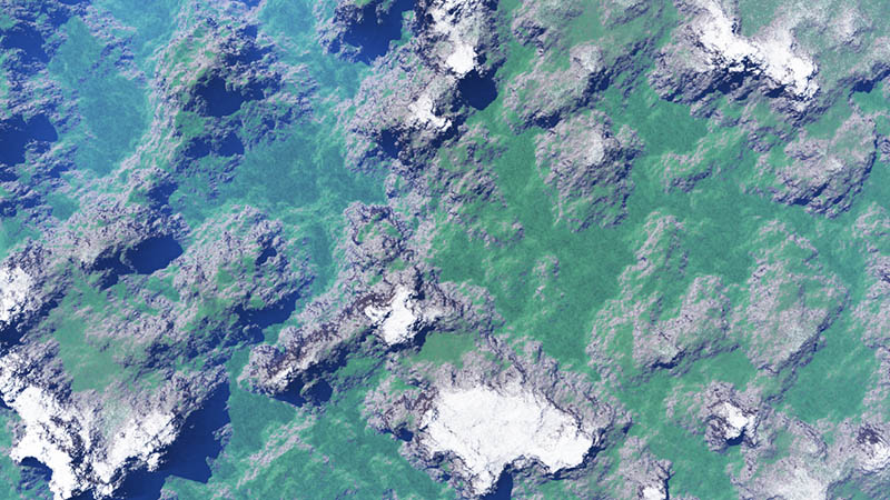
While this is obviously not a physically realistic algorithm, it goes a long way towards producing realistic-looking terrain. As can be seen from the following top-down view,
there are no preferred directions (the view is axis-aligned).
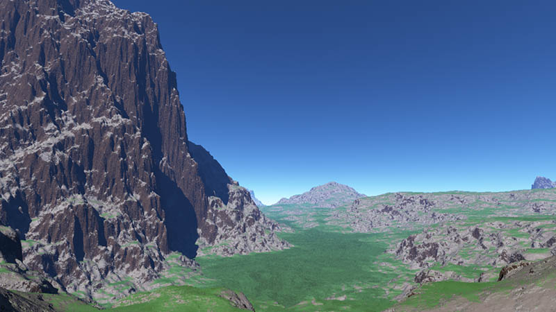
The view below shows that the algorithm is capable of generating both steep cliffs and realistic flat valleys. The valley shown is not a local minimum, but in fact slopes gently down towards the single minimum of the map. You can also see that the algorithm in fact generates terrain as steep as the underlying heighfield representation can handle. There is naturally some stretching on the cliff faces, simply because the steepness of the terrain is approaching the maximum that can be represented by a regular heighfield.
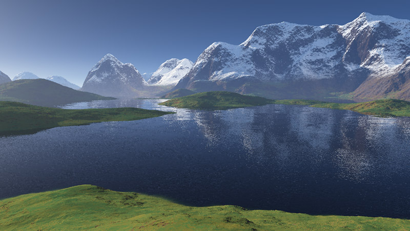
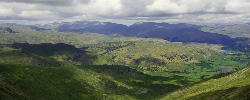
Here is an aerial view of the same map, put next to a photograph of heavily glaciated terrain from the English lake district. As you can see, many of the same terrain features are present in both (although the fractal landscape in this case is more rugged, perhaps closer to the terrain that would be expected in Greenland).
Fixing Stationarity
To generate landscapes with differing properties in different locations, we can vary something called the crossover scale of the landscape. The crossover scale is the scale of subdivision where we begin to displace grid points. It defines the maximum vertical scale of a terrain.
It just so happens that we have the perfect way of varying this: we can use another fractal function to decide the crossover scale of the map. Places where this function approaches a maximum value, we start fractal behaviour earlier, and get high mountains. Places where this function approaches an intermediate value, we start fractal behaviour later, and get rolling hills. And places where it approaches a minimum value, we get flat plains. The result is then called a multi-fractal.
Note that when using this technique, you need to use upwards-only displacement in the generation, otherwise you will end up with mountain valleys lower than the surrounding plains.
Repeating Landscapes
Provided we do everything on a regular square grid, there is nothing to stop us making a landscape wrap around, so that it repeats infinitely. This is particularly useful if we want to add detail at different scales. In an idea world, we could generate a landscape thousands of kilometres across, with detail down to the millimetre level. Unfortunately, computers aren't big enough to store all that data. We can, however, approximate the same effect by overlaying a larger landscape with a repeating detail landscape. This requires support in the rendering step for doing this, but most rendering packages will have this functionality.
Erosion
Once you have a landscape free of statistical issues, you can apply hydrological and thermal erosion models to further modify the landscape. You can also simulate water flow to build river networks and so on. Often erosion is considered a post-processing step, but in reality it is much more efficient to do it at multiple scales in-line with the generation of the landscape. A discussion of possible algorithms for this is below.
Stochastic Fractal Object Placement
Suppose now that we want to place trees, plants, and other natural objects in our generated landscape. These will have a naturally varying distribution, depending on the dynamics of the landscape. If, for example, water is a constraint, we would only want to put trees where our hydrological model says there will be water. If altitude is a constraint, we'd only want the trees to grow at lower altitudes, and in any case only on ground where the gradient is lower. All these constraints can be expressed as a continuously varying density function across the landscape (essentially a probability density function).
Once we have such a function, placing the objects is easy: we integrate the function for all positions in the landscape. Then we choose a random number within the range of the integral function, and use the function to look up the corresponding position. Thus we can just use random numbers, and have the trees appear at the correct locations.
The same approach can be used for bushes, grass, rocks and any other objects that belong in the landscape.
Useful post-processing Transformations
Generally, we want to constrain the height ranges of the generated surface. This is easily done by normalizing the surface. For a floating point surface, you might normalize in the range of 0..1. Then it is simple to apply scaling transforms on export, with the added plus that we can combine multiple fractal surfaces by averaging or multiplication without affecting the overall height range.
One useful post-processing step that can have a significant impact on the generated landscape is to apply some simple per-point transforms to the generated heightfield. The most obvious of these is a quick-and-dirty "glaciation" where we just square the height values of the normalized (0..1) heights. This has the effect of making the slopes steeper and the mountains more pointed.
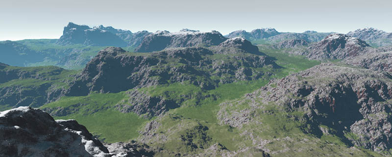
The above image shows all the details discussed here. The flat ground between the mountains (occupied by the shallow lake) is a consequence of the modified Dijkstra algorithm. The low hills around there have been flattened by a glaciation post-processing transform. Equally, the mountains have been made steeper and more irregular by the horizontal fractal displacement and by the subsquent glaciation transform. Also note that the landscape has no preferred directions, with planar and curving cliffs running in all directions.

Erosion Models
So far, I've focused on methods for generating terrain using fractal subdivision and displacement. I've also explored a number of ways to fix the common issues these landscapes exhibit. One thing I did not do was explore post-processing erosion models. Traditionally, these models have been applied to achieve a number of different effects, which are not possible without.
These effects, common to natural landscapes, but lacking from procedurally generated ones are:
- The in-filling of local minima, to better approximate natural terrain.
- The formation of Talus slopes as observed in, for example, desert environments (e.g. sand dunes).
- The creation of gradient discontinuities in landscapes (e.g. ridges).
Of these, the first one is already better dealt with using the modified Dijkstra method above. This leaves the formation of Talus slopes and the formation of ridges.
Models of Thermal Erosion
The classic model of thermal erosion used in landscape synthesis is dh/dt(p) = -k * (slope(p) - tan(talus_angle)). This is often used to approximate all non-hydrological erosion. In other words, the erosion at a point is proportional to the amount by which the gradient exceeds the talus angle. The talus angle is usually set globally - valid values run from around 30 to 45 degrees. The classical thermal model also re-deposits the eroded material downslope.
Using this equation repeatedly on a regular grid can, however, lead to a number of diagonally-aligned and axis-aligned artefacts that we would want to avoid. In order to achieve visually better results, we can use the sum of the slope between a point all all points downslope of it. If the slope sum exceeds twice the talus gradient, the point is eroded proportionally to that difference. The material is then re-deposited downhill to all points whose slope relative to the point exceed the talus gradient, in proportion to the amount by which it was exceeded. If this doesn't make any sense, bear with me, the equations are in the next section.
This produces an erosion scheme with no preferred directions, that makes talus slopes of constant gradient, generally without numerical artefacts. Eagle-eyed readers may spot that this is non-conservative, in that sometimes a point might be eroded without deposition, although unless the point is a local maximum, this is unlikely.
Problems with Thermal Erosion in Alpine Environments
There are several problems with this simple model. One is that all cells will be eroded equally, but another more significant problem is that it takes no account of the way in which Talus may be carried away by other erosive processes. This is particularly significant in alpine regions, where glaciers, avalanches and high-speed water runoff will carry away eroded material.
To compensate for this, I use a model of alpine erosion where there is zero deposition of the eroded material. So we remove material that would be eroded in the above scheme, but never deposit it. This produces a far better fit to the observed characteristics of temparate mountain environments than the classical model. It also erodes backwards into steep areas effectively, which produces results that are similar to the glacial erosion seen in these environments. In particular, it is capable of creating sharp ridges without leaving huge piles of talus everywhere.
Formally:
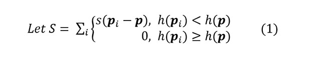
S is the sum of downhill slopes.
p is the point we calculate the erosion for
pi are the 8 neighbouring points.
h(p) is the height of point p
s(pi - p) is minus the partial derivative of height h(p) from p to pi.
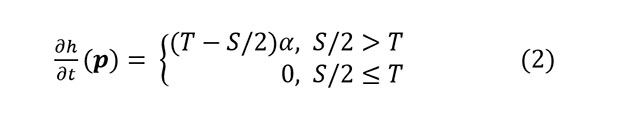
dh/dt(p) is the rate of change of height of point p over time.
T is the talus gradient, i.e. tan(theta) where theta is the talus angle.
S is the slope sum from equation 1.
alpha is a global relaxation parameter - I set this to 0.25
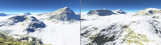
Both erosion models use the same formulation, but in the case of my implementation of thermal erosion, material removed from p is then distributed to any neighbours where s(pi - p) is greater than T, in proportion to s(pi - p) - T. The alpine erosion model just discards the material. A comparison of the results of these two models is shown below. In particular, notice how the alpine model erodes further into cliffs, resulting in the ridges that we would expect to find in an alpine landscape.
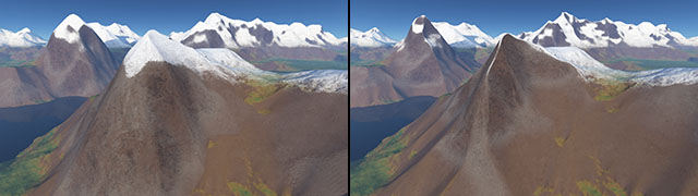
The image on the left shows 125 iterations of classical thermal erosion. The image on the right shows 125 iterations of alpine erosion. Both are rendered in Terragen without adding fractal detail, so that shape of the resulting terrain can be seen. The picture below shows how the terrain is affected by the number of iterations of alpine erosion applied.
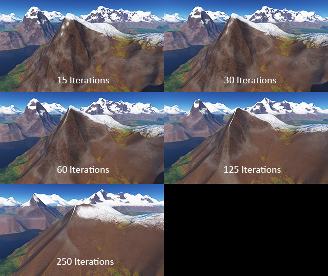
Clearly, using erosion will remove fractal detail - if the scheme being used is numerically stable, it will result in smooth slopes where erosion has taken place. It is therefore a good idea to add this detail back in afterwards. Terragen has a feature that automatically adds small-scale fractal detail to surfaces, but this would be easy enough to implement in any package - you just apply a repeating fractal surface at smaller scale.
Modifying Erosion to Account For Altitude
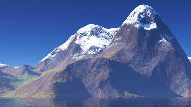
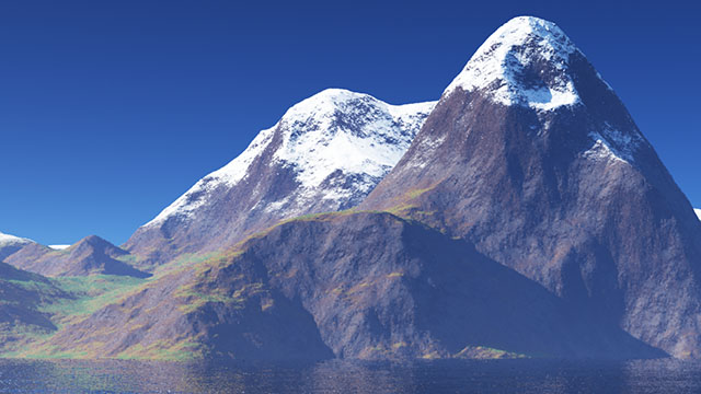
A further simple but effective change is to modify the amount of erosion according to the altitude. This simulates the increased strength of alpine erosive processes at higher altitudes. The pictures below show the same mountain, before and after 60 iterations of alpine erosion. Both have been rendered with Terragen, with fractal detail added to the surface afterwards. You can see that the erosion has sharpened the ridges that were more rounded in the original landscape.
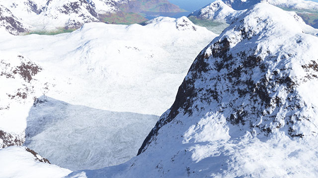
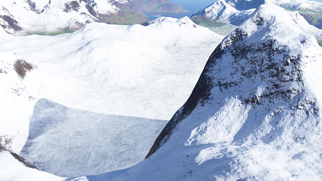
Lastly, here is a comparison of the effects of altitude-dependent erosion. The first image is a detail of a mountain after 40 iterations of altitude-independent erosion. You can see that the details in the lower terrain features have been eroded substantially. The second image is the same detail, of the same mountain, after 60 iterations of altitude-dependent erosion. You can see that the details of the higher mountain areas are the same, but the lower terrain features have retained more fractal detail.
The code used to generate these terrains was written in C# - I will make the source available on Github and as a Nuget package in the future. Feel free to extend and modify the code to suit your needs.
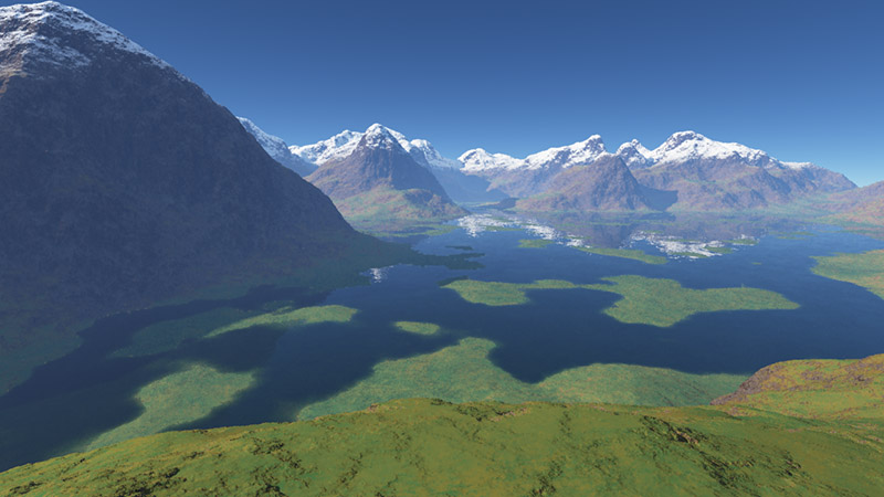
The above picture shows all features discussed in this and the previous section. The shallow water covers a Dijkstra plain, although the base level of the terrain here is about halfway between the global minimum and the tops of the mountains. Without the lake, water would flow in the direction the camera is looking, towards the global minimum which is just in front of the two mountains in the far distance on the left. The mountains have been eroded with 60 iterations of altitude-dependent alpine erosion, and thus are showing the classic ridges and faces that we expect to see in alpine environments.
Catmull-Rom Splines, Cubic surfaces and Interpolating Subdivision
Because of the importance of splines in generating fractal landscapes, I thought I might present some additional notes on how to interpolate grid points using efficient subdivision schemes. For those of you not interested in the methods, here is a summary of the results:
Catmull Rom Cubic Coefficients
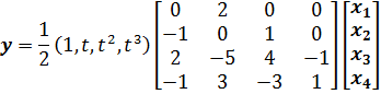
The cubic catmull-rom spline is given by:
Where y is the result vector, t is the parameter (between 0 and 1) and x(n) are the grid vectors. In other words, we have 4 points, x1...x4 and we're trying to interpolate smoothly between the middle two, x2 and x3. At t=0, the above equation evaluates to y = x2, and at t=1, it evaluates to x3. Intermediate values give points in-between.
1-Dimensional Cubic subdivision
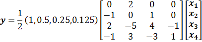
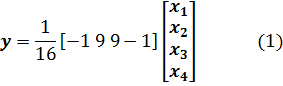
Evaluating this at t=0.5 gives us a cubic approximation for the midpoint of x2 and x3, which is exactly what we need for subdivision:
This is the cubic approximation for the midpoint of x2 and x3.
2-Dimensional Cubic subdivision
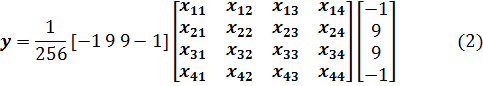
To obtain a 2-D subdivision scheme, we just multiply the coefficient vector of the 1-dimensional scheme by a 4x4 point matrix, and then by the 1-d vector again:
This gives us an expression for the midpoint of the interior 4 points, in terms of the surrounding 16 points.
Bi-cubic resampling
Therefore, to up-sample the entire landscape by 2 (prior to fractal perturbation), all you have to do is apply (1) to the top edge and the left edge, and apply (2) to get the midpoint of each patch. If you have a repeating landscape (which is the easiest choice), then the values simply wrap around at the edges.
How do derive it all
I'm not going to do a rigorous mathematical derivation of all this, because I don't really want to write that much. However, the basic sketch goes as follows:
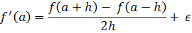
- Write out the taylor series expansions of f(a+h) and f(a-h)
- Re-arrange each of them in terms of f'(a)
- Combine the two equations to cancel the error terms. This gives you a 3-point derivative operator:
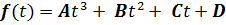
- Write down the generalized cubic:
- Observe that for gradient continuity at the endpoints of the x2...x3 interval, the following conditions must be true:
- At t=0, f(t) = x2
- At t=1, f(t) = x3
- At t=0, f'(t) = h2
- At t=0, f'(t) = h3
Where h2 and h3 are the gradients at x2 and x3.
- Observe that the formula from 3) can be used to replace h2 and h3 with combinations of the points x1...x4.
- Use the conditions to form a set of 4 simultaneous equations, and solve for the coefficients A, B, C and D
The end result of this process is the equation for the cubic Catmull-Rom spline that we started with.
|